Anaconda
A conda package is a compressed tarball file that
contains system-level libraries, Python or other modules, executable
programs and other components. Conda keeps track of the
dependencies between packages and platforms.
凡使用 pip install
安装的包均为编译安装, conda install
安装的则为编译好的二进制包.
conda 包可以打包其他语言, pip 包容易出现系统依赖问题
conda 包的依赖管理更完善
conda 环境下仍可使用 pip 进行安装, 但所使用的 pip 命令和系统中的 pip
互不影响, 安装的包的位置也在 conda 本身的目录下.
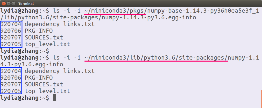
每个环境互不影响, 各环境下的包虽然必须分别安装 (也可以 clone
一个现有环境),hard link .
(更多讨论参考 https://jakevdp.github.io/blog/2016/08/25/conda-myths-and-misconceptions/)
使用
三个部分:
root
/usr usr user
/home/<user>/.local .local anaconda/miniconda
/home/<user>/miniconda3 miniconda3 conda 目录结构 (安装之后自动修改了软连接,
修改环境变量后系统优先使用这个位置)
/home/<user>/miniconda3/ pkgs/ bin/ python -> python3.6
│ ├── python3 -> python3.6
│ ├── python3.6
│ ├── jupyter
│ ├── h5dump
│ └── ...
├── include/ lib/ share/ envs env1/ bin/ include/ lib/ share/ env2/
IPython & Jupyter
参考文档 http://jupyter-notebook.readthedocs.io/en/stable/
一般用户配置文件在 ~/.jupyter
config:
    /home/lydia/.jupyter
    /home/lydia/miniconda3/etc/jupyter
    /usr/local/etc/jupyter
    /etc/jupyter
data:
    /home/lydia/.local/share/jupyter
    /home/lydia/miniconda3/share/jupyter
    /usr/local/share/jupyter
    /usr/share/jupyter
runtime:
/run/user/1000/jupyter1 2 %run script.py %run script.ipynb
1 2 3 %%sh cd ~/miniconda3/pwd
/home/lydia/miniconda3可以看到实际并未改变当前目录 (因为是子进程):
'/home/lydia/codes/zly/python/python-intro'1 2 3 %%script idl cd, current=d print , d
/home/lydia/codes/zly/python/python-intro
IDL Version 8.2.1 (linux x86_64 m64). (c) 2012, Exelis Visual Information Solutions, Inc.
逐行使用 bash 命令 (注意不加 '!' 的区别):
得到的结果可以存入变量:
1 2 current, = !pwd current
'/home/lydia/python-intro'下面这两句不能写在一个 Cell 中:
'/home/lydia/miniconda3'用 {var} (推荐) 或 $var (不推荐) 调用当前
ipython 环境的变量:
/home/lydia/codes/zly/python/python-intro/home/lydia/codes/zly/python/python-intro/home/lydia/codes/zly/python/python-intro见 http://mmcdan.github.io/posts/interacting-with-the-shell-via-jupyter-notebook/
1 2 3 4 a = 1 b = 'x' %whos int str
Variable Type Data/Info
----------------------------
a int 1
b str x语法细节
python2 & python3
1 2 3 %%python2 print 1 / 2 print 1 // 2
0
01 2 3 %%python3 print (1 / 2 )print (1 // 2 )
0.5
0详见 Python 2 -> 3 的转换
list,
tuple
对 list 或 tuple, 当只有一个元素时, 注意加逗号:
listlistinttuple
赋值, 星号 (*) 表达式用来展开 list/tuple, 双星号
(**) 用来展开 dict (常用于函数参数表):
1 2 a, b, *c = [0 , 1 , 2 , 3 ] a, b, c
(0, 1, [2, 3])0dict
dict 改变某个 key 但 value 不变的方法
1 2 3 d = {'a' : 1 , 'b' : 2 } d['c' ] = d.pop('b' ) d
{'a': 1, 'c': 2}1 2 d1 = {'a' : 1 , 'b' : 2 } d2 = {'a' : -1 , 'c' : 3 , 'd' : 4 }
{'a': -1, 'b': 2, 'c': 3, 'd': 4}1 dict (list (d1.items()) + list (d2.items()))
{'a': -1, 'b': 2, 'c': 3, 'd': 4}{'a': -1, 'b': 2, 'c': 3, 'd': 4}set
{1, 2, 3}{1, 2, 3, 4, 5}{2, 3, 4, 5}{2, 3, 4, 5}
set 求交集, 并集, 差集, 对称差集, 子集
1 {1 , 2 }.intersection({2 , 3 })
{2}{2}{1, 2, 3}{1, 2, 3}1 {1 , 2 }.difference({2 , 3 })
{1}{1}1 {1 , 2 }.symmetric_difference({2 , 3 })
{1, 3}{1, 3}TrueTrue1 {1 , 2 }.issubset({1 , 2 , 3 })
TrueTrue1 {1 , 2 , 3 }.issuperset({1 , 2 })
TrueTrue一些特性的演示
插件 https://github.com/lgpage/nbtutor http://pythontutor.com/
1 2 3 %%nbtutor -r -f l1= (0 ) l2 = (0 ,)
网页版演示
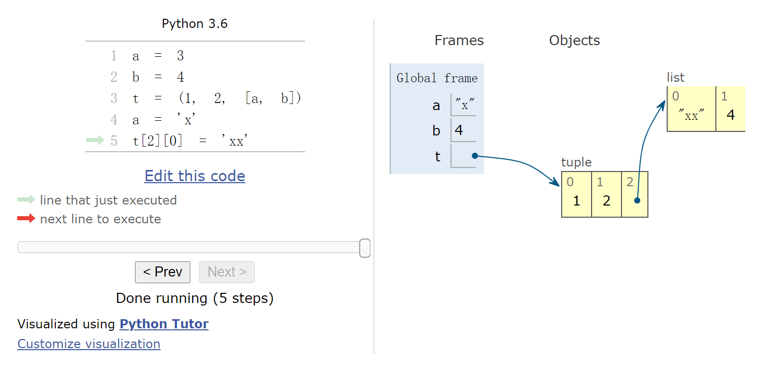
1 2 3 4 5 6 %%nbtutor -r -f -i a = 3 b = 4 t = (1 , 2 , [a, b]) a = 'x' t[2 ][0 ] = 'xx'
(1, 2, ['xx', 4])网页版演示
包含判断的单行循环
1 2 l = [1 , 2 , 3 , 4 , 5 ] [i for i in l if i > 2 ]
[3, 4, 5]例如用 globals() 来得到字符串形式的变量名 (python
的变量没有提供这个功能的关键字, 因为"变量名"存储在namespaces中)
1 2 3 4 5 6 def namestr (obj, namespace ): return [name for name in namespace if namespace[name] is obj][0 ] a = 1 b = 2 for var in (a, b): print (f'{namestr(var, globals ())} = {var} ' )
a = 1
b = 2单行 if (三元关系运算)
1 2 3 a = 1 b = 'y' if a > 0 else 'n' b
'y'循环, 迭代器, 生成器
Python 的 for 循环不使用索引变量, 而使用遍历迭代器
(iterator) 的方式处理可迭代对象 (range, set 等):
遍历的方式是使用 iter 和 next 函数:
0[0, 1, 2, 3, 4]enumerate 函数适合需要同时使用索引和内容时使用:
1 2 3 for i, item in enumerate (l): i = ... item = ...
生成器:
1 2 a = (i**2 for i in range (5 )) a
<generator object <genexpr> at 0x14da87e652b0>41 2 a = [i for i in range (3 )] a
[0, 1, 2]1 2 tuple (i for i in range (3 ))
(0, 1, 2)函数定义
1 2 3 4 def func (a, b, *args, **kwargs ): ... return ...
1 2 3 def f (x, y ): return x + y f(1 , 2 )
3用 lambda 语法来定义:
1 2 f = lambda x, y: x + y f(1 , 2 )
31 (lambda x, y: x + y)(1 , 2 )
3命名空间和变量作用域
https://sebastianraschka.com/Articles/2014_python_scope_and_namespaces.html
globals() 以 dict 形式返回当前所有全局变量,
包括导入的包名, ipython/jupyter 的 In, Out
等.
True1 2 3 4 5 6 7 i = 1 def f (): i = 2 print (i, 'local' ) return f() print (i, 'global' )
2 local
1 global1 2 3 4 i = 1 for i in range (4 ): pass i
31 2 3 i = 1 [i for i in range (3 )] i
1有关函数中的变量作用方式细节, 参考这里提到的例子: stackoverflow
Any time you see varname
= creating a new name binding
within the function's scope.varname was
bound to before is lost within this scope.
Any time you see
varname.foo() calling a method on varname. The method
may alter varname (e.g. list.append). varname (or, rather, the object that varname
names) may exist in more than one scope, and since it's the same object,
any changes will be visible in all scopes .
NumPy
numpy 的数据类型 dtype
https://www.tutorialspoint.com/numpy/numpy_data_types.htm
1 2 3 4 5 6 >>> np.dtype(np.int64) is np.dtype('i8' ) is np.dtype('<i8' )True >>> np.dtype(np.int64) is np.dtype('int' ) is np.dtype('int64' )True >>> np.dtype(np.int64) is np.dtype('>i8' )False
1 2 3 4 >>> np.dtype(np.float64) is np.dtype('f8' ) is np.dtype('<f8' )True >>> np.dtype(np.float64) is np.dtype('float' ) is np.dtype('float64' )True
Fortran 二进制文件读写 中的应用.
np.arange 参数为浮点数时要注意的细节
array([0. , 0.3, 0.6, 0.9, 1.2, 1.5])array([0. , 0.3, 0.6, 0.9, 1.2, 1.5, 1.8, 2.1])'2.1000000000000001'看一个求和的例子中同样的问题 (用 list 和
numpy.ndarray 效果一样):
1 2 3 4 5 6 7 8 print ('%.17f' % 0.1 )print ('%.17f' % sum ([0.1 ] * 10 ))import mathprint ('%.17f' % math.fsum([0.1 ] * 10 ))
0.10000000000000001
0.99999999999999989
1.00000000000000000False1 math.fsum([0.1 ] * 10 ) == 1
True1 math.fsum([0.1 ] * 10 ) == 1.0
True参考 https://docs.python.org/3/tutorial/floatingpoint.html
建议是: 使用整数; 对浮点数的情况, stop 值设得略小一些
(比如减去步长的一般) 以防止改点被包含, 或使用 np.linspace
代替.
矩阵
np.matrix(矩阵) 是 np.ndarray(数组)
的一个子类, 继承了父级的方法, 也定义了新的方法 (例如矩阵运算).
1 issubclass (np.matrix, np.ndarray)
True1 a = np.matrix([[0 , 1 , 2 ], [3 , 4 , 5 ]]); a
matrix([[0, 1, 2],
[3, 4, 5]])1 a = np.matrix("0 1 2; 3 4 5" ); a
matrix([[0, 1, 2],
[3, 4, 5]])numpy.matrixlib.defmatrix.matrixnp.asmatrix (或简写作 np.mat) 相当于
np.matrix(data, copy=False)
1 2 3 4 x = np.array([[1 , 2 ], [3 , 4 ]]) m = np.matrix(x) m[0 , 0 ] = 5 x
array([[1, 2],
[3, 4]])1 2 3 4 x = np.array([[1 , 2 ], [3 , 4 ]]) m = np.mat(x) m[0 , 0 ] = 5 x
array([[5, 2],
[3, 4]])1 x.__array_interface__['data' ][0 ] == m.__array_interface__['data' ][0 ]
True注意: np.matrix 既是一个类名也是一个函数名, 而
np.mat, np.asmatrix 只是函数名.
数组和矩阵运算
数组运算
1 a = np.arange(12 ).reshape(3 , -1 ); a
array([[ 0, 1, 2, 3],
[ 4, 5, 6, 7],
[ 8, 9, 10, 11]])11array([[ 0, 1, 4, 9],
[ 16, 25, 36, 49],
[ 64, 81, 100, 121]])array([[ 0, 1, 4, 9],
[ 16, 25, 36, 49],
[ 64, 81, 100, 121]])使用数组进行矩阵运算
scipy.linalg 与 numpy.linalg 的比较: https://scipy.github.io/devdocs/tutorial/linalg.html
>* scipy.linalg contains all the
functions in numpy.linalg plus some other more
advanced ones not contained in
numpy.linalg * Despite its convenience, the use of the
numpy.matrix class is discouraged . *
scipy.linalg operations can be applied
equally to numpy.matrix or to 2D
numpy.ndarray objects.
1 a = np.diagflat([1. , 2. , 3. ]); a
array([[1., 0., 0.],
[0., 2., 0.],
[0., 0., 3.]])1 b = np.array([[-1. , -1. , -1. ],[0. , 0. , 0. ]]); b
array([[-1., -1., -1.],
[ 0., 0., 0.]])1 2 from scipy.linalg import invinv(a)
array([[ 1. , 0. , -0. ],
[ 0. , 0.5 , -0. ],
[ 0. , 0. , 0.33333333]])array([[-1., 0.],
[-2., 0.],
[-3., 0.]])直接使用矩阵类型进行运算
使用 numpy 的矩阵类型 numpy.matrix
1 a = np.mat(np.diagflat([1. , 2. , 3. ])); a
matrix([[1., 0., 0.],
[0., 2., 0.],
[0., 0., 3.]])1 b = np.mat(np.array([[-1. , -1. , -1. ],[0. , 0. , 0. ]])); b
matrix([[-1., -1., -1.],
[ 0., 0., 0.]])matrix([[-1., 0.],
[-2., 0.],
[-3., 0.]])matrix([[-1., 0.],
[-2., 0.],
[-3., 0.]])matrix([[ 1. , 0. , -0. ],
[ 0. , 0.5 , -0. ],
[ 0. , 0. , 0.33333333]])用作坐标格点的数组的几种形式
1 2 3 4 5 6 7 8 9 10 11 12 13 14 15 16 >>> x = np.linspace(0 , 2 , 3 ); xarray([ 0. , 1. , 2. ]) >>> y = np.linspace(3 , 6 , 4 ); yarray([3. , 4. , 5. , 6. ]) >>> X, Y = np.meshgrid(x, y)>>> X array([[0. , 1. , 2. ], [0. , 1. , 2. ], [0. , 1. , 2. ], [0. , 1. , 2. ]]) >>> Yarray([[3. , 3. , 3. ], [4. , 4. , 4. ], [5. , 5. , 5. ], [6. , 6. , 6. ]])
可用来计算坐标的函数 (例如磁场的表达式等等, 见 examples/streamplot.py
) 1 2 3 4 U = (np.cos(k1 * X) * np.exp(-k1 * Y) - np.cos(k2 * X) * np.exp(-k2 * Y)) V = (- np.sin(k1 * X) * np.exp(-k1 * Y) + np.sin(k2 * X) * np.exp(-k2 * Y))
1 2 3 4 x = np.linspace(0 , 2 , 3 ) y = np.linspace(3 , 6 , 4 ) X, Y = np.meshgrid(x, y, indexing='ij' ) Y.shape
(3, 4)j 标记默认是虚数单位,
但在这里表示前面的数字是格点数.nn*1j + 1j, 1不能省
(否则j定义为变量)np.ogrid 可参见 numpy
相关文档
1 2 3 4 5 6 7 8 9 10 11 12 13 14 15 16 17 18 19 20 >>> x = np.linspace(0 , 2 , 3 )>>> y = np.linspace(3 , 6 , 4 )>>> X, Y = np.mgrid[0 :2 :3j , 3 :6 :4j ]>>> X, Y = np.array([i.astype(np.float64) for i in np.mgrid[0 :3 , 3 :7 ]])>>> X, Y = np.array(np.meshgrid(x, y, indexing='ij' ))>>> X array([[0. , 0. , 0. , 0. ], [1. , 1. , 1. , 1. ], [2. , 2. , 2. , 2. ]]) >>> Y array([[3. , 4. , 5. , 6. ], [3. , 4. , 5. , 6. ], [3. , 4. , 5. , 6. ]])
mask
1 a = np.arange(9 ).reshape(3 , -1 ); a
array([[0, 1, 2],
[3, 4, 5],
[6, 7, 8]])array([[False, False, False],
[False, False, True],
[ True, True, True]])(array([1, 2, 2, 2]), array([2, 0, 1, 2]))1 list (zip (*np.where(a > 4 )))
[(1, 2), (2, 0), (2, 1), (2, 2)]array([[ 0, 1, 2],
[ 3, 4, -1],
[-1, -1, -1]])其他对数组元素的处理
处理含有 NaN 的数据:
e.g. 求最值可使用 np.nanmin(...) 和
np.nanmax(...)
Matplotlib
1 2 3 fig = plt.gcf() ax = plt.gca() im = plt.gci()
得到当前 backend: 1 2 >>> import matplotlib.pyplot as plt>>> plt.get_backend()
1 2 >>> import maplotlib as mpl>>> mpl.get_backend()
选择 backend (在导入其他 matplotlib 模块之前):
1 2 >>> import matplotlib>>> matplotlib.use('TkAgg' )
用户配置文档 matplotlibrc~/.config/matplotlib/matplotlibrc (Linux)
用 zorder 来控制图层:
这个例子中也展示了加入一个动态的竖线的方法,
这条线在保存后的图像中不会显示.
1 2 %matplotlib %run -e 'examples/test_plot.py'
1 2 %matplotlib %run -e 'examples/test_imshow.py'
命令行脚本: examples/test_imshow_click.py
(jupyter 中无法使用)
SunPy
示例
示例文件
注意: 这些例子只是提供一个使用参考, 不一定是最优的.
示例中的 fits 读取方法
更多 FITS 的读取方法参见 Python
简易教程#FITS-文件读取 Astropy
的命令行工具
读取HMIMap 的例子:
1 2 3 4 import sunpy.map smap = sunpy.map .Map('data/hmi.B_720s.20150827_052400_TAI.field.fits' ) type (smap)
sunpy.map.sources.sdo.HMIMap这是 GenericMap 的一个子类:
1 2 issubclass (sunpy.map .sources.sdo.HMIMap, sunpy.map .mapbase.GenericMap)True
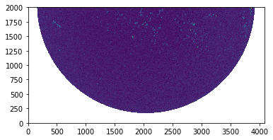
Truenumpy.ndarray(4096, 4096)smap.data[i, j] 中的 i 为 Y 轴, 单位为 pixel:
1 2 3 import matplotlib.pyplot as pltplt.imshow(smap.data[0 :2000 , :], origin='lower' ); plt.show()
png
关于 Scaled Image Data
这一部分将更仔细地检查 Astropy 对示例中的 FITS 文件的处理.
参见 http://docs.astropy.org/en/stable/io/fits/usage/image.html#scaled-data
Images are scaled only when either of the BSCALE/BZERO keywords are
present in the header and either of their values is not the default
value (BSCALE=1, BZERO=0).
由于 astropy.io.fits 的特性, 读取 'Scaled Image Data'
时, 调用 .data 将自动对数据进行缩放: 1 physical value = BSCALE * (storage value) + BZERO
astropy.io.fits.open 中使用
do_not_scale_image_data=True 可禁用这一步骤.
见 astropy.io.fits
FAQ
数据类型:
BITPIX
Numpy Data Type
8
numpy.uint8 (unsigned integer)
16
numpy.int16
32
numpy.int32
-32
numpy.float32
-64
numpy.float64
可以使用 Astropy 的命令行工具在 shell 中查看信息:
1 2 fname = 'data/hmi.B_720s.20150827_052400_TAI.field.fits' !fitsinfo {fname}
Filename: data/hmi.B_720s.20150827_052400_TAI.field.fits
No. Name Ver Type Cards Dimensions Format
0 PRIMARY 1 PrimaryHDU 6 ()
1 1 CompImageHDU 155 (4096, 4096) int32 可以看到该文件存储的数据类型是整形.
用命令行工具查看关键字 'BITPIX':
1 !fitsheader -e 1 --keyword BITPIX {fname}
# HDU 1 in data/hmi.B_720s.20150827_052400_TAI.field.fits:
BITPIX = 32 / data type of original image 使用 astropy.io.fits:
1 2 3 from astropy.io import fitshdulist = fits.open (fname) hdu = hdulist[1 ]
32'BSCALE' 不为零则为 'scaled':
0.010.01 hdulist.verify('silentfix+warn' )
dtype('float64')142.83nan-64手动 scale:
'BSCALE' 虽然之前已被删除, 但值仍存储在 ._orig_bscale
中. .scale 将使用这个值.
0.01014283-214748364832使用 SunPy 处理时, 'BITPIX', 'BSCALE', 'BZERO' 的值被保留,
.data 仍进行了 scale 的过程.
针对不同文件, 如果 SunPy 的程序内部使用 astropy.io.fits
处理文件时调用了 .data 再返回 header, 即
astropy.io.fits 已经如上所述改变了 header, 那么 SunPy
所返回的 header 中 'BITPIX', 'BSCALE', 'BZERO' 可能已经被改变.
下面的例子中得到的 header 是最初的值:
1 2 import sunpy.map smap = sunpy.map .Map('data/hmi.B_720s.20150827_052400_TAI.field.fits' )
320.010.0142.83320.010.0坐标和单位
SunPy map http://docs.sunpy.org/en/stable/code_ref/map.html#using-map-objects
>A number of the properties of this class are
returned as two-value named tuples that can either be -
indexed by
position: [0] , [1] .x , .y .axis1 , .axis2
PixelPair(x=<Quantity 4096. pix>, y=<Quantity 4096. pix>)\(4096 \; \mathrm{pix}\)
\(\mathrm{pix}\)
4096.0astropy.units 的使用方法:
1 import astropy.units as u
\(\mathrm{\mathring{A}}\)
\(4096 \; \mathrm{pix}\)
\([4096,~4096] \; \mathrm{pix}\)
1 smap.dimensions.x.unit is u.pix
True/home/lydia/miniconda3/lib/python3.6/site-packages/sunpy/map/mapbase.py:669: Warning: Missing metadata for heliographic longitude: assuming longitude of 0 degrees
lon=self.heliographic_longitude,
astropy.coordinates.sky_coordinate.SkyCoord[<Quantity 0. pix>, <Quantity 0. pix>]1 smap.pixel_to_world(*(4096 , 4096 ) * u.pix)
<SkyCoord (Helioprojective: obstime=2015-08-27 05:22:21.800000, rsun=696000000.0 m, observer=<HeliographicStonyhurst Coordinate (obstime=2015-08-27 05:22:21.800000): (lon, lat, radius) in (deg, deg, m)
(0., 7.089004, 1.51196988e+11)>): (Tx, Ty) in arcsec
(-1040.36199634, -1030.86554911)>查看 SkyCoord 的帮助:
1 2 import astropy.coordinateshelp (astropy.coordinates.sky_coordinate.SkyCoord)
\(\mathrm{-7.65399^{\prime\prime}}\)
1 smap.pixel_to_world(*(2000 , 2000 ) * u.pix)
<SkyCoord (Helioprojective: obstime=2015-08-27 05:22:21.800000, rsun=696000000.0 m, observer=<HeliographicStonyhurst Coordinate (obstime=2015-08-27 05:22:21.800000): (lon, lat, radius) in (deg, deg, m)
(0., 7.089004, 1.51196988e+11)>): (Tx, Ty) in arcsec
(16.55031204, 26.53575639)>1 smap.pixel_to_world(*(2000 , 2000 ) * u.pix).transform_to('heliographic_stonyhurst' )
<SkyCoord (HeliographicStonyhurst: obstime=2015-08-27 05:22:21.800000): (lon, lat, radius) in (deg, deg, km)
(1.00568591, 8.68202918, 696000.0000022)>查看坐标信息:
/home/lydia/miniconda3/lib/python3.6/site-packages/sunpy/map/mapbase.py:669: Warning: Missing metadata for heliographic longitude: assuming longitude of 0 degrees
lon=self.heliographic_longitude,
<Helioprojective Frame (obstime=2015-08-27 05:22:21.800000, rsun=696000000.0 m, observer=<HeliographicStonyhurst Coordinate (obstime=2015-08-27 05:22:21.800000): (lon, lat, radius) in (deg, deg, m)
(0., 7.089004, 1.51196988e+11)>)>出现这个 Warning 时:
1 2 smap.meta['hgln_obs' ] = 0. ; smap.meta['hgln_obs' ] = 0. ; smap.meta['hgln_obs' ] = 0. smap.coordinate_frame
<Helioprojective Frame (obstime=2015-08-27 05:22:21.800000, rsun=696000000.0 m, observer=<HeliographicStonyhurst Coordinate (obstime=2015-08-27 05:22:21.800000): (lon, lat, radius) in (deg, deg, m)
(0., 7.089004, 1.51196988e+11)>)>语法对比
比较 plothmi.py 与对应 IDL 程序的语法:
下面的语句中, 为了简便和方便对比, 使用了自定义的一些函数. 导入方法:
1 from usr_sunpy import read_sdo, plot_map, plot_vmap, image_to_helio
读取数据 1 2 3 ; IDL read_sdo,<fname>,index,data index2map,index,data,mapa
1 2 3 mapa = read_sdo(<fname>)
旋转 1 2 3 4 5 ; IDL ; 2 表示180° mapbx.data = rotate(mapbx,2) mapby.data = rotate(mapbx,2) mapbz.data = rotate(mapbx,2)
1 2 3 4 5 mapbx = mapbx.rotate(order=1 ) mapby = mapby.rotate(order=1 ) mapbz = mapbz.rotate(order=1 )
截取 1 2 3 4 ; IDL sub_map,mapbx,smapbx,xrange=[500,800.0],yrange=[-500,-100.0] sub_map,mapby,smapby,ref_map=smapbx sub_map,mapbz,smapbz,ref_map=smapbx
1 2 3 4 5 6 7 bl = SkyCoord(500 *u.arcsec, -500 *u.arcsec, frame=mapbz.coordinate_frame) tr = SkyCoord(800 *u.arcsec, -100. *u.arcsec, frame=mapbz.coordinate_frame) smapbx = mapbx.submap(bl, tr) smapby = mapby.submap(bl, tr) smapbz = mapbz.submap(bl, tr)
绘图 1 2 3 ; IDL plot_map,smapbz,dmax=2000,dmin=-2000,color=0,charsize=1.8,... plot_vmap,/over,smapbx,smapby,mapbz=smapbz,limit=180,scale=0.012,iskip=15,jskip=15,...
1 2 3 4 5 6 fig = plt.figure() ax = fig.add_subplot(111 , projection=smapbz) plot_map(ax, smapbz) plot_vmap(ax, smapbx, smapby, smapbz, iskip=iskip, jskip=jskip, cmin=100. , vmax=500. , cmap='binary' , ...)
坐标变换 1 2 ; IDL ; magnetic_modeling_codes/.../05projection_modified_version.pro
1 2 3 4 5 6 7 8 hx, hy = image_to_helio(smapbz) smapbx_h, smapby_h, smapbz_h = image_to_helio(smapbx, smapby, smapbz) plot_map(ax, smapbz_h, coords=(hx, hy)) plot_vmap(ax, smapbx_h, smapby_h, smapbz_h, coords=(hx, hy), ...)
插值,
拟合
选择不限于这里列举的包, 以后也可能会有更合适的方法出现.
相关安装见 Python 安装和配置
插值
求极值
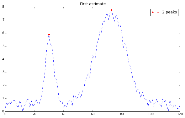
官方例图
(http://peakutils.readthedocs.io/en/latest/tutorial_a.html):
1 2 import peakutilsindexes = peakutils.indexes(y, thres=0.5 , min_dist=30 )
Enhancing the resolution by interpolation: 1 peaks_x = peakutils.interpolate(x, y, ind=indexes)
拟合
LMFIT (Non-Linear Least-Squares Minimization and Curve-Fitting)
下载 https://github.com/lmfit/lmfit-py
文档 http://lmfit.github.io/lmfit-py/
有现成模型, 也可以自定义模型.examples/lmfits
(来自 LMFIT网站示例
)
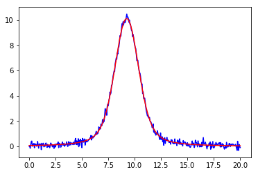
使用内置模型:
1 2 3 4 5 6 7 8 9 10 11 12 13 from lmfit.models import GaussianModel data = np.loadtxt('test_peak.dat' ) x = data[:, 0 ] y = data[:, 1 ] mod = GaussianModel() pars = mod.guess(y, x=x) out = mod.fit(y, pars, x=x) print (out.fit_report()) plt.plot(x, out.init_fit, 'k--' ) plt.plot(x, out.best_fit, 'r-' )
1 2 %matplotlib inline %run examples/lmfits/fit_peak.py
[[Model]]
Model(voigt)
[[Fit Statistics]]
# fitting method = leastsq
# function evals = 21
# data points = 401
# variables = 4
chi-square = 10.9301767
reduced chi-square = 0.02753193
Akaike info crit = -1436.57602
Bayesian info crit = -1420.60017
[[Variables]]
sigma: 0.89518909 +/- 0.01415450 (1.58%) (init = 0.8775)
center: 9.24374847 +/- 0.00441903 (0.05%) (init = 9.25)
amplitude: 34.1914737 +/- 0.17946860 (0.52%) (init = 65.43358)
gamma: 0.52540198 +/- 0.01857955 (3.54%) (init = 0.7)
fwhm: 3.22385343 +/- 0.05097475 (1.58%) == '3.6013100*sigma'
height: 10.0872204 +/- 0.03482130 (0.35%) == 'amplitude*wofz((1j*gamma)/(sigma*sqrt(2))).real/(sigma*sqrt(2*pi))'
[[Correlations]] (unreported correlations are < 0.100)
C(sigma, gamma) = -0.928
C(amplitude, gamma) = 0.821
C(sigma, amplitude) = -0.651
png
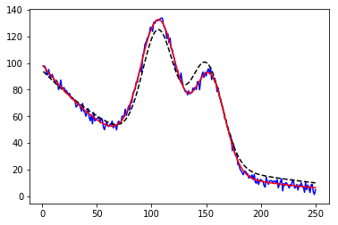
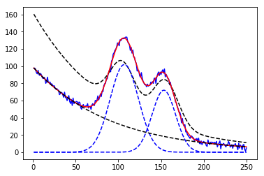
多个模型叠加:
1 2 3 4 5 6 7 8 9 10 11 12 13 14 15 16 17 18 19 20 21 22 23 from lmfit.models import ExponentialModel, GaussianModeldata = np.loadtxt('NIST_Gauss2.dat' ) x = data[:, 0 ] y = data[:, 1 ] exp_mod = ExponentialModel(prefix='exp_' ) gauss1 = GaussianModel(prefix='g1_' ) gauss2 = GaussianModel(prefix='g2_' ) pars1 = exp_mod.guess(y, x=x) pars2 = gauss1.guess(y, x=x) pars3 = gauss2.guess(y, x=x) pars = pars1 + pars2 + pars3 mod = gauss1 + gauss2 + exp_mod out = mod.fit(y, pars, x=x) print (out.fit_report())plt.plot(x, y, 'b' ) plt.plot(x, out.init_fit, 'k--' ) plt.plot(x, out.best_fit, 'r-' )
1 2 3 %%capture output %matplotlib inline %run examples/lmfits/fit_peaks.py
png
1 2 3 %%capture output %matplotlib inline %run examples/lmfits/fit_peaks_components.py
png
自定义模型的方法见 LMFIT网站示例
其他
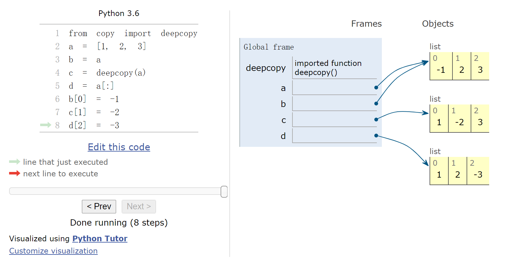
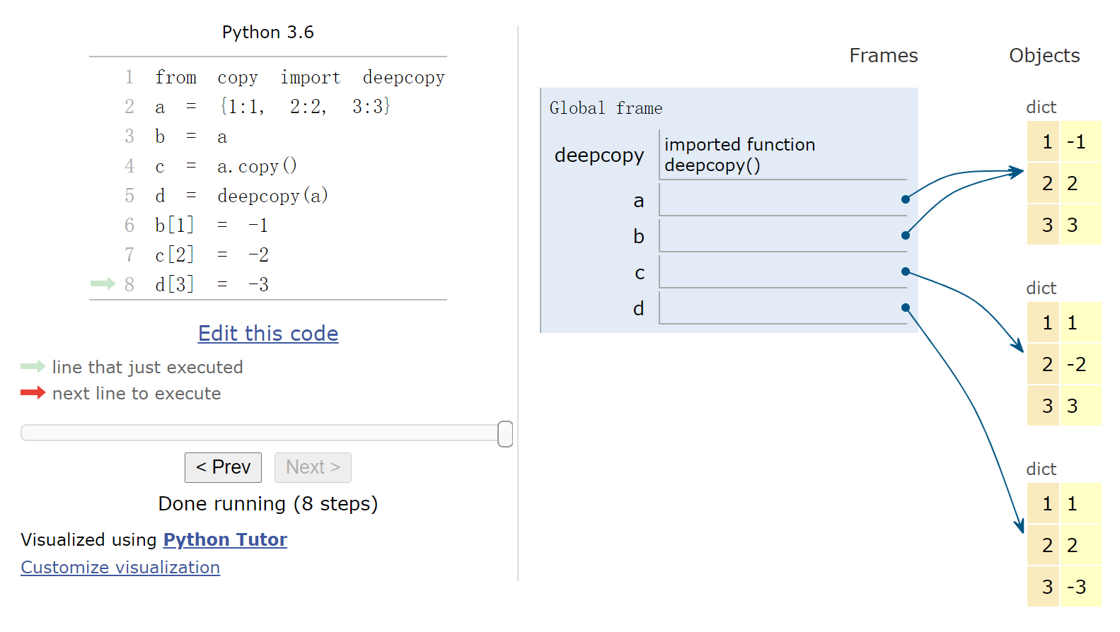
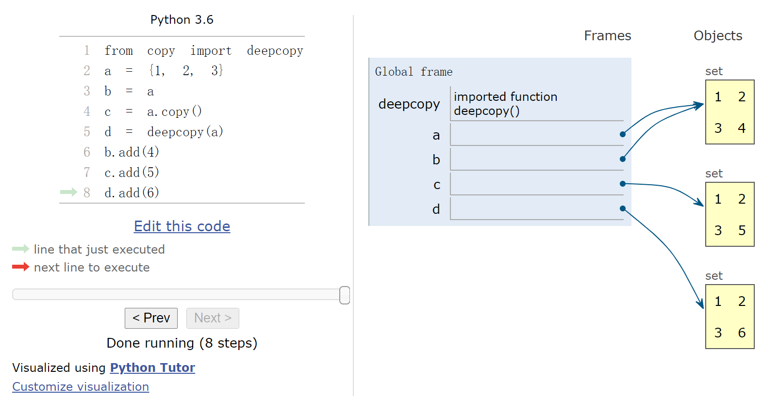
copy 注意事项
"shallow copy" vs "deep copy"
演示插件 https://github.com/lgpage/nbtutor
1 2 3 4 5 6 7 8 9 %%nbtutor -r -f -i from copy import deepcopya = [1 , 2 , 3 ] b = a c = deepcopy(a) d = a[:] b[0 ] = -1 c[1 ] = -2 d[2 ] = -3
1 print (id (a), id (b), id (c), id (d))
23284866388232 23284866388232 23284855519880 23284856061064网页版演示
1 2 3 4 5 6 7 8 9 %%nbtutor -r -f -i from copy import deepcopya = {1 :1 , 2 :2 , 3 :3 } b = a c = a.copy() d = deepcopy(a) b[1 ] = -1 c[2 ] = -2 d[3 ] = -3
1 print (id (a), id (b), id (c), id (d))
22492371132064 22492371132064 22492397510376 22492397507280网页版演示
1 2 3 4 5 6 7 8 9 %%nbtutor -r -f -i from copy import deepcopya = {1 , 2 , 3 } b = a c = a.copy() d = deepcopy(a) b.add(4 ) c.add(5 ) d.add(6 )
1 print (id (a), id (b), id (c), id (d))
22492476895528 22492476895528 22492476895304 22492374233384网页版演示
1 2 3 4 5 6 7 8 9 %%nbtutor -r -f -i import numpy as npa = np.arange(1 , 4 ) b = a[:] c = a.copy() d = a[[0 , 2 ]] b[0 ] = -1 c[1 ] = -2 d[1 ] = -3
1 2 3 for i in (a, b, c, d): print (id (i), i.__array_interface__['data' ][0 ])
22928831926400 93879086511872
22928831928960 93879086511872
22928829201984 93879072448320
22928829199344 93879078700736网页版演示 (Site
Error : Ruby and Python+Anaconda backends are permanently
unavailable)
参见之前的 np.matrix, np.asmatrix
其他格式文件读写
用 pandas 读 csv
1 2 3 import pandas as pddata = pd.read_csv("data/data.csv" ) data
col1
col2
col3
0
row1
1
10.0
1
row2
2
0.2
2
row3
3
300.0
Index(['col1', 'col2', 'col3'], dtype='object')0 row1
1 row2
2 row3
Name: col1, dtype: object0 row1
1 row2
2 row3
Name: col1, dtype: object只取一部分:
1 2 data = pd.read_csv("data/data.csv" , nrows=2 , usecols=(0 ,2 )) data
col1
col3
0
row1
10.0
1
row2
0.2
对于超大文件, 参见: https://www.dataquest.io/blog/pandas-big-data/
Fortran 二进制文件读写
使用 scipy.io.FortranFilehttps://docs.scipy.org/doc/scipy-0.15.1/reference/generated/scipy.io.FortranFile.read_record.html
1 2 3 4 5 6 7 8 9 10 11 12 13 14 15 16 17 from scipy.io import FortranFilevar1 = 1.1 var2 = 0 arr = np.arange(6. ).reshape((2 , 3 )) print (var1, var2)print (arr)print (f'arr[0, 1] = {arr[0 , 1 ]} ' )with FortranFile('data/data_fortran1-1.dat' , 'w' ) as f: f.write_record(var1) f.write_record(var2) f.write_record(arr) with FortranFile('data/data_fortran1-2.dat' , 'w' ) as f: f.write_record(var1, var2, arr)
1.1 0
[[0. 1. 2.]
[3. 4. 5.]]
arr[0, 1] = 1.01 2 3 4 5 6 7 8 9 10 11 12 13 14 15 16 17 18 19 from scipy.io import FortranFilewith FortranFile('data/data_fortran1-1.dat' , 'r' ) as f: var1 = float (f.read_record('<f8' )) var2 = int (f.read_record('<i8' )) arr = f.read_record('(2, 3)<f8' ) print ('data_fortran1-1.dat' )print (var1, var2)print (arr)with FortranFile('data/data_fortran1-2.dat' , 'r' ) as f: data = f.read_record([('var1' , '<f8' ), ('var2' , '<i8' ), ('arr' , '(2, 3)<f8' )]) print ('\ndata_fortran1-2.dat' )print (f'keys = {data.dtype.names} ' ) print (float (data['var1' ]), int (data['var2' ]))print (data['arr' ])
data_fortran1-1.dat
1.1 0
[[0. 1. 2.]
[3. 4. 5.]]
data_fortran1-2.dat
keys = ('var1', 'var2', 'arr')
1.1 0
[[[0. 1. 2.]
[3. 4. 5.]]]1 2 3 4 %%bash cd examples/ifort -o test_read_seq test_read_seq.f90 ./test_read_seq
data_fortran1-1.dat
1.1 0.0
0.0 1.0 2.0
3.0 4.0 5.0
arr(2, 1) = 1.0
data_fortran1-2.dat
1.1 0.0
0.0 1.0 2.0
3.0 4.0 5.0
arr(2, 1) = 1.0见 Structured arrays: https://docs.scipy.org/doc/numpy/user/basics.rec.html
struct 参考 https://docs.python.org/3/library/struct.html
1 2 3 4 5 6 7 8 9 10 11 12 import structvar1 = 1.1 var2 = 0 arr = np.arange(6. ).reshape((2 , 3 )) print (var1, var2)print (arr)print (f'arr[0, 1] = {arr[0 , 1 ]} ' )with open ('data/data_fortran2.dat' , 'wb' ) as f: f.write(struct.pack('d' , var1)) f.write(struct.pack('i' , var2)) arr.tofile(f)
1.1 0
[[0. 1. 2.]
[3. 4. 5.]]
arr[0, 1] = 1.01 2 3 4 5 6 7 8 with open ('data/data_fortran2.dat' , 'rb' ) as f: var1 = float (np.fromfile(f, dtype='<f8' , count=1 )) var2 = int (np.fromfile(f, dtype='<i4' , count=1 )) arr = np.fromfile(f, dtype='<f8' ).reshape(2 , 3 ) print (var1, var2)print (arr)
1.1 0
[[0. 1. 2.]
[3. 4. 5.]]1 2 3 4 %%bash cd examples/ifort -o test_read_stream test_read_stream.f90 ./test_read_stream
1.1 0.0
0.0 1.0 2.0
3.0 4.0 5.0
arr(2, 1) = 1.0HDF5
文件读写, NCDF, CDF 文件读取
读写 HDF5
文件, 读 NCDF 文件
HDF5 格式介绍 https://portal.hdfgroup.org/display/HDF5/Introduction+to+HDF5
相关包: h5py 或 pandas +
pytables
(http://www.pytables.org/usersguide/datatypes.html)
安装见 Python 安装和配置
1 2 $ h5dump -H <filename>.hdf5 $ ncdump -h <filename>.ncdf
1 2 3 4 5 6 7 8 import h5pyarr = np.arange(10000 ).reshape(50 ,-1 ) with h5py.File('test.hdf5' , 'w' ) as f: f['data' ] = arr f['lb' ] = list (range (100 ))
读纯 HDF5/NCDF 文件: 1 2 3 4 f = h5py.File('test.hdf5' , 'r' ) keys = list (f.keys()) items = list (f.items()) a = f['data' ].value
1 2 3 4 5 6 a = f['data' ]['block0_values' ].value f.close()
1 2 3 from pprint import pprintpprint([(f'{k:>20 } ' , f'{str (f[k].shape):>20 } ' , f'{str (f[k].dtype):>20 } ' ) for k in f.keys()]) pprint([(f'{k:>20 } ' , f"{str (f[k]['block0_values' ].shape):>20 } " , f"{str (f[k]['block0_values' ].dtype):>20 } " ) for k in f.keys()])
写: 1 2 3 4 5 arr2 = pd.DataFrame(arr) with pd.HDFStore('test2.hdf5' , 'w' ) as f: f['data' ] = arr2 f['lb' ] = pd.DataFrame(list (range (100 )))
1 2 3 4 5 f = pd.HDFStore('test2.hdf5' , 'r' ) keys = f.keys() items = list (f.items()) a = f.data.values f.close()
读纯 HDF5/NCDF 文件:.root
1 2 3 4 5 6 7 8 f = pd.HDFStore('test.hdf5' , 'r' ) keys = list (f.root._v_children.keys()) items = list (f.root._v_children.items()) a = f.root.data.read() f.close()
打印 (以免数据有 None, 用 np.shape): 1 2 3 4 pprint([(f'{k} ' .rjust(20 ), f'{np.shape(f.get_node(k))} ' .rjust(20 ), f'{np.dtype(f.get_node(k))} ' .rjust(20 )) for k in list (f.root._v_children.keys())])
H5T_STRING
大小比较
用于比较的文件名说明:
Filename
Method
xxx _np.npynp.save
xxx _np.npznp.savez_compressed
xxx _compimg.fitsFITS CompImageHDU
(compressed)
xxx _prim.fitsFITS PrimaryHDU
xxx _h5py_0.hdf5h5py
xxx _h5py_gzip.hdf5h5py
xxx _h5py_lzf.hdf5h5py
xxx _pd_0.hdf5pandas
xxx _pd_blosc.hdf5pandas
xxx _pd_bzip2.hdf5pandas
xxx _pd_lzo.hdf5pandas
xxx _pd_zlib.hdf5pandas
1 2 3 4 5 6 7 %run examples/test_hdf5.py print ()!du -h data/test_*.np* print ()!du -h data/test_h5py_*.hdf5 print ()!du -h data/test_pd_*.hdf5
array: 15.3 M
7.7M data/test_np.npy
1.3M data/test_np.npz
16M data/test_h5py_0.hdf5
2.9M data/test_h5py_gzip.hdf5
7.7M data/test_h5py_lzf.hdf5
16M data/test_pd_0.hdf5
272K data/test_pd_blosc.hdf5
248K data/test_pd_bzip2.hdf5
256K data/test_pd_lzo.hdf5
172K data/test_pd_zlib.hdf51 2 3 4 5 6 7 %run examples/test_hdf5_2.py print ()!du -h data/test_*.np* print ()!du -h data/test_h5py_*.hdf5 print ()!du -h data/test_pd_*.hdf5
array: 15.3 M
7.7M data/test_np.npy
7.2M data/test_np.npz
16M data/test_h5py_0.hdf5
8.0M data/test_h5py_gzip.hdf5
9.5M data/test_h5py_lzf.hdf5
16M data/test_pd_0.hdf5
7.7M data/test_pd_blosc.hdf5
7.2M data/test_pd_bzip2.hdf5
7.7M data/test_pd_lzo.hdf5
7.1M data/test_pd_zlib.hdf51 2 3 4 5 6 7 8 9 10 11 12 fname = 'data/hmi.B_720s.20150827_052400_TAI.field.fits' %run examples/test_fits_hdf5.py {fname} print ()!du -h {fname} print ()!du -h data/fits_*.np* print ()!du -h data/fits_*.fits print ()!du -h data/fits_h5py_*.hdf5 print ()!du -h data/fits_pd_*.hdf5
array: 64.0 M
21M data/hmi.B_720s.20150827_052400_TAI.field.fits
65M data/fits_np.npy
27M data/fits_np.npz
21M data/fits_compimg.fits
65M data/fits_prim.fits
65M data/fits_h5py_0.hdf5
27M data/fits_h5py_gzip.hdf5
40M data/fits_h5py_lzf.hdf5
65M data/fits_pd_0.hdf5
23M data/fits_pd_blosc.hdf5
21M data/fits_pd_bzip2.hdf5
23M data/fits_pd_lzo.hdf5
20M data/fits_pd_zlib.hdf51 2 3 4 5 6 7 8 9 10 11 12 fname = 'data/hmi.B_720s.20150827_052400_TAI.disambig.fits' %run examples/test_fits_hdf5.py {fname} print ()!du -h {fname} print ()!du -h data/fits_*.np* print ()!du -h data/fits_*.fits print ()!du -h data/fits_h5py_*.hdf5 print ()!du -h data/fits_pd_*.hdf5
array: 32.0 M
5.4M data/hmi.B_720s.20150827_052400_TAI.disambig.fits
33M data/fits_np.npy
5.2M data/fits_np.npz
5.4M data/fits_compimg.fits
33M data/fits_prim.fits
33M data/fits_h5py_0.hdf5
5.3M data/fits_h5py_gzip.hdf5
9.7M data/fits_h5py_lzf.hdf5
33M data/fits_pd_0.hdf5
9.5M data/fits_pd_blosc.hdf5
4.1M data/fits_pd_bzip2.hdf5
7.6M data/fits_pd_lzo.hdf5
4.8M data/fits_pd_zlib.hdf5读取 CDF 文件
相关包 cdflib, 安装见 Python 安装和配置#其他
1 2 3 4 5 6 import cdflibf = cdflib.CDF("<filename>.cdf" ) f.cdf_info() f.varinq('<key>' ) f.varget('<key>' ) f.close()
NumPy to VTK
参考 https://pyscience.wordpress.com/2014/09/06/numpy-to-vtk-converting-your-numpy-arrays-to-vtk-arrays-and-files/ Python 安装和配置 examples/field2dvtk.py
,
Matlab mat 文件读写
(未测试) 1 2 3 4 5 import scipy.ioscipy.io.loadmat("<filename>" , mdict=None , appendmat=True , **kwargs) scipy.io.savemat("<filename>" , mdict, appendmat=True , format ='5' , long_field_names=False , do_compression=False , oned_as='row' )
脚本相关
脚本结构
文件头:
脚本结构: 1 2 3 4 5 6 7 8 9 10 11 12 13 14 15 16 17 18 19 20 21 22 23 24 25 26 """ 假设这个文件的名称为 mymodule.py 使用 `imort mymodule` 导入 这些文字会出现在 `help(mymodule)` 或 `pydoc mymodule` 中 """ c = 1 def func1 (x, y, *args, **kwargs ): """ 这个注释必须缩进 args: a tuple - (arg1, arg2, ...) kwargs: a dict - {key1 : val1, key2 : val2} """ global c return x + y + c def func2 (x ): a = func1(x, x) return a def _func3 (x ): pass return def main (): if __name__ == "__main__" : main()
import 这个文档时,
__name__ 为模块名, 因此 main() 不执行
help() 也可以查看模块内的函数文档:
1 2 import usr_sunpyhelp (usr_sunpy.plot_map)
try ... except ... 语法
1 2 3 4 5 6 7 8 9 10 try : ... except ValueError as e: print ('ValueError:' , e) except ZeroDivisionError as e: print ('ZeroDivisionError:' , e) else : print ('no error!' ) finally : print ('finally...' )
见 Paraview 的例子
Paraview 脚本
官方文档 https://www.paraview.org/ParaView/Doc/Nightly/www/py-doc/index.html
1 from paraview.simple import *
也可以使用文件头 #!/usr/bin/env pvbatch,
加执行权限后直接执行:
1 2 view = GetActiveView() scene = GetAnimationScene()
view.ViewTime 修改时 scene.AnimationTime
不变 scene.AnimationTime 修改时 view.ViewTime
也同时被改变
注意: filter 必须是显示状态 (Show(<filter>))
才能修改时间
1 2 !code -n examples/stat1.py
字体选择参考路径:
/usr/share/fonts/truetype/dejavu/DejaVuSans.ttf
/home//miniconda3/lib/python3.6/site-packages/matplotlib/mpl-data/fonts/ttf/DejaVuSans.ttf
python 调用问题 (paraview 5.5.0+ 没有这个问题):
paraview 某个版本之后就默认使用 python 2.7.11+.PYTHONPATH 和
PYTHONSTARTUP), 1 2 3 4 #!/bin/bash unset PYTHONSTARTUP export PYTHONPATH=/<your_path>/ParaView/lib/python2.7/site-packages/<your_path>/ParaView/bin/paraview $@
paraview,
pvpython 和 pvbatch 命令.
Python 2 -> 3 的转换
比较推荐的安全的检查方式:
备份的原文件且自动生成转换过的文件
手动比较, 在需要的地方对照修改 filename.bakfrom __future__ import division, print_function1 2 $ sudo apt-get install meld $ meld filename filename.bak
确认无误后, 将手动修改的文件复制回去 1 $ mv -v filename.bak filename
python 内查看版本的方法, 可用于 if 语句等 (更推荐用
try...except... 语法):
1 2 3 import sysprint (sys.version_info >= (3 , 0 ))print (sys.version_info.major >= 3 )
执行 shell 命令
https://docs.python.org/3/library/subprocess.html
1 2 3 4 5 6 7 8 9 10 11 import subprocessfname = 'installpy.ipynb' subprocess.run(["ls" , "-l" , fname]) print (subprocess.run(["ls" , "-l" , fname], stdout=subprocess.PIPE) .stdout.decode('ascii' )) print (subprocess.check_output(["ls" , "-l" , fname]).decode('ascii' ))
-rw-rw-r-- 1 lydia lydia 142508 Jun 24 16:21 installpy.ipynb
-rw-rw-r-- 1 lydia lydia 142508 Jun 24 16:21 installpy.ipynb利用 bash 的特长来做一些字符串操作:
1 2 3 4 5 6 7 8 9 fname_head = subprocess.check_output(r"echo -n %s | sed 's/\.ipynb//'" % fname, shell=True ).decode('ascii' ) fname_head = subprocess.check_output(r"echo %s | sed 's/\.ipynb//'" % fname, shell=True ).strip().decode('ascii' ) print (fname_head)
installpy字符串编码见 廖雪峰的网站
'/home/lydia/codes/zly/python/python-intro'1 os.path.split(os.path.abspath(__file__))[0 ]
或 1 os.path.dirname(os.path.abspath(__file__))
其中 os.path.split 和 os.path.dirname
的用法:
1 os.path.split('your/path/filename' )
('your/path', 'filename')1 os.path.dirname('your/path/filename' )
'your/path'os.path.dirname 类似于 bash 的 dirname
1 !dirname 'your/path/filename'
your/path脚本选项
推荐 argparse, 在过去的其他方法的基础上有所增强 https://docs.python.org/3/library/argparse.html
脚本内: 1 2 3 4 5 6 7 8 9 import argparseparser = argparse.ArgumentParser(description='Process some integers.' ) parser.add_argument('integers' , metavar='N' , type =int , nargs='+' , help ='an integer for the accumulator' ) parser.add_argument('--sum' , dest='accumulate' , action='store_const' , const=sum , default=max , help ='sum the integers (default: find the max)' ) args = parser.parse_args() print (args.accumulate(args.integers))
1 2 3 4 5 6 7 8 $ python prog.py -h usage: prog.py [-h] [--sum] N [N ...] Process some integers. positional arguments: N an integer for the accumulator optional arguments: -h, --help show this help message and exit --sum sum the integers (default: find the max)
处理 warnings
1 2 3 4 5 6 7 8 9 10 11 12 13 14 with np.errstate(invalid='ignore' ): ... ... import warningswith warnings.catch_warnings(): warnings.simplefilter("ignore" ) ... ... warnings.simplefilter("ignore" , category=xxx) ... ...
urllib, requests
示例和文件来自 http://python4astronomers.github.io
注意 python3 不再使用 urllib2
1 2 3 4 5 6 7 8 9 10 11 12 13 14 15 16 17 import urlliburl = 'http://python4astronomers.github.io/_downloads/myidlfile.sav' urllib.request.urlretrieve(url, 'myidlfile.sav' ) with open ('myidlfile.sav' , 'wb' ) as f: f.write(urllib.request.urlopen(url).read()) import requestswith open ('myidlfile.sav' , 'wb' ) as f: f.write(requests.get(url).content) import requestsr = requests.get(<url>) with open (filename, 'wb' ) as f: for chunk in r.iter_content(chunk_size=128 ): f.write(chunk)